Monday (7/19) Response

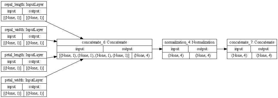
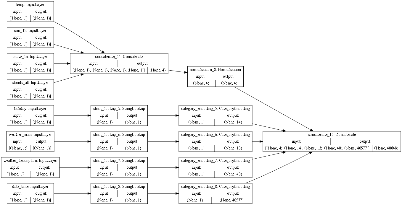
(1) Use the plot_model() command from tf.keras.utils to produce the plot that describes the input preprocessing step. Describe the plot of each model for the two dataset preprocessing steps.
What does each box in the illustration represent? Are there different paths towards the final concatenation step? What is occurring at each step and why is it necessary to execute before fitting your model.

• This is the plot that represents the preprocessing steps for the iris dataset. The first set of boxes shows all the features in their current states. Since all the variables are continuous there is only one path from this point forward. Moving on to the second group, this is where the first concatenation step happens. This means that all the features are consolidated into one string. After this normalization occurs followed by another concatenation step.

• The traffic volume preprocessing steps are represented by the plot above. Just like the iris dataset the first group is all the features of the dataset prior to being altered. Unlike the prior dataset this data contains several categorical variables that must be treated differently than the continuous variables. As can be seen in the plot, all the categorical variables avoid the first concatenation step and instead partake in string lookup which is then followed by category encoding. Both of these alternative steps lead to these features being converted into dummy variables. This means that in this dataset there are indeed multiple paths that lead to the final concatenation step.

• To give slightly more detail on why each step is important, without concatenation the different features would not be merged into one string, making it difficult to run a model. The normalization step is then vital to make sure these merged strings are of a common scale. This allows the model to be more accurate. Then a final concatenation step occurs to account for any features that may have not been included in the first concatenation step due to them being categorical variables. The alternative steps that convert those categorical variables into dummy variables are vital because they allow for all features to be numerical and consistent.

(2) Train each model and produce the output (not necessary to validate or test).
Describe the model output from each of the trained metro traffic interstate dataset and the iris flowers dataset.

-Iris Model:

Epoch 1/10
4/4 [==============================] - 0s 3ms/step - loss: 1.1921e-07
Epoch 2/10
4/4 [==============================] - 0s 0s/step - loss: 1.1921e-07
Epoch 3/10
4/4 [==============================] - 0s 0s/step - loss: 1.1921e-07
Epoch 4/10
4/4 [==============================] - 0s 3ms/step - loss: 1.1921e-07
Epoch 5/10
4/4 [==============================] - 0s 342us/step - loss: 1.1921e-07
Epoch 6/10
4/4 [==============================] - 0s 3ms/step - loss: 1.1921e-07
Epoch 7/10
4/4 [==============================] - 0s 0s/step - loss: 1.1921e-07
Epoch 8/10
4/4 [==============================] - 0s 3ms/step - loss: 1.1921e-07
Epoch 9/10
4/4 [==============================] - 0s 3ms/step - loss: 1.1921e-07
Epoch 10/10
4/4 [==============================] - 0s 3ms/step - loss: 1.1921e-07 

• Consisting of ten epochs this model produced rather odd results. The loss remained stagnant throughout every epoch and the model completed extraordinarily fast. It could be argued that the loss is just so small that differences can’t be seen but I doubt that is the case. All in all, much more time should be put into this model to attempt to create the best results.

-Traffic Volume Model:

Epoch 1/10
1507/1507 [==============================] - 23s 15ms/step - loss: 12192317.0000
Epoch 2/10
1507/1507 [==============================] - 26s 17ms/step - loss: 5628457.5000
Epoch 3/10
1507/1507 [==============================] - 27s 18ms/step - loss: 3836894.2500
Epoch 4/10
1507/1507 [==============================] - 26s 17ms/step - loss: 3744486.2500
Epoch 5/10
1507/1507 [==============================] - 26s 17ms/step - loss: 3702563.0000
Epoch 6/10
1507/1507 [==============================] - 26s 17ms/step - loss: 3665475.7500
Epoch 7/10
1507/1507 [==============================] - 26s 17ms/step - loss: 3630548.5000
Epoch 8/10
1507/1507 [==============================] - 26s 17ms/step - loss: 3596066.0000
Epoch 9/10
1507/1507 [==============================] - 26s 17ms/step - loss: 3561109.7500
Epoch 10/10
1507/1507 [==============================] - 26s 17ms/step - loss: 3525196.5000

• Similar to the previous model this model had a very odd output. The loss is decreasing, but it is significantly higher than it should be. Once again, more time should be put into this model if the goal was to produce the best model.

(3) What is the target for each dataset?

• The target for the iris dataset is to correctly identify the species of iris the plant is. The three potential options being setosa, versicolor, and virginica. The data points for the target classify as categorical variables.

• The target for the second dataset is the volume of traffic present. This target data consists of continuous variables

(4) How would you assess the accuracy of each model?

• The accuracy for the iris dataset was either really impressive, or not accurate. The loss remained the same at each epoch at an extremely low figure. I assume the change in loss is either so small that it cannot be noticed, or there is some sort of issue within the model that needs to be addressed.

• The accuracy for the model of the traffic volume dataset is abysmal, with a massive loss of 3525196.5 by the 10th and final epoch.

(5) Are you using a different metric for each one? Why is this so? What is each one measuring?

• For the iris dataset Categorical Crossentropy was the metric used. This is simply due to the target being a categorical variable. This metric does pretty exactly much what the name declares it does, calculate the crossentropy loss between the labels and predictions. This makes it the ideal metric for this dataset.

• In the Traffic volume dataset the metric used to measure the loss is mean squared error. This is the most efficient metric due to the target consisting of continuous variables as previously stated. MSE works by calculating the mean distance between the actual y and the y predicted value, which is useful because it makes it easy to determine how far off the model was from correctly identifying the correct y value.